
Sculpting noise with dynamical bias
Photonic qubits have the great advantage that they don’t easily interact with their environment and hence are intrinsically less noisy than many other qubit types. But this reclusiveness also makes entangling photonic qubits a nondeterministic process. No matter how perfectly photonic components are fabricated, there’s always a chance that entangling operations may not perform as hoped. But crucially, we receive a clear indication of when a photonic entangling operation fails. This is quite a different from noise in other types of qubits – which easily sneaks by unnoticed. You might say that whereas matter-based qubits are dishonest, photons are merely disobedient.
Our recent work on Dynamic Bias Arrangement 1] makes good use of this silver lining. The (nondeterministic) entangling operation we use in our fault tolerant photonic quantum computer are called fusions, which are essentially two-outcome entangling measurements. Not only can we know when fusions fail, we can furthermore steer, or bias, precisely where these failures occur. By dynamically biasing our fusion measurements we minimize the impact of their nondeterminism and improve our error correcting capabilities.
In the rest of this post we will describe the idea behind these dynamic bias arrangements in a little more detail. But first let’s get to grips with fusion operations and how they relate to fault tolerance.
Fusing photons
In fusion based quantum computing small, entangled resource states are joined together via networks of fusion operations acting on their constituent photons. For example, Figure 1 shows a fusion network joining 4 photon resource states (resource states shown in black, fusions shown in gray).
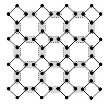
Figure 1: Illustrative example of a simple fusion network from a fusion based quantum computation. In this example 4-photon small, entangled resource states (black diamonds) are further joined by a regular network of fusion measurements (shown shaded gray). See [2] for more details.
1. The fusion network shown in is a pedagogical example only. More complex networks are considered in 1] and more generally for actual fault tolerant quantum computations.
Each fusion operation performs both an XX and ZZ measurement on two photonic qubits. Consequently, each fusion produces two binary measurement outcomes – one for the XX measurement and one for the ZZ.
Fusion networks can be carefully constructed such that we expect certain subsets of these measurements to have an even parity in the absence of errors. Monitoring these kind of parity checks between fusion outcomes allow the detection of errors.
But as we’ve already mentioned, fusion operations are nondeterministic. Both the XX and ZZ measurements of a fusion operation only get successfully performed 50% of the time. In the other 50% of cases, we experience a fusion failure – wherein only one of the two measurements is correctly performed.
This seems like a pretty dire occurrence – on average we’re losing 25% of our desired measurement outcomes! However, we can tweak the circuit implementing a fusion such that we can choose, or bias, whether it’s the XX or ZZ measurement which fails[2]. With this ability we can cleverly bias each fusion so that any failure has the most benign possible effect on our error correcting capabilities.
Syndrome graphs
To decide how we should bias any given fusion measurements we need to make use of a visualization known as the syndrome graph. This helps us keep track of how measurement outcomes contribute to the parity checks we use to detect errors.
A syndrome graph represents parity checks[3] as nodes. Each node connects a number of edges – which represent the measurement outcomes contributing to that parity check as we fuse together a network of resource states. The values of these parity checks are processed by a decoder algorithm, which tries to work backwards to infer which edges (i.e. which fusions) must have experienced errors. Importantly, this use of parity checks allows us to detect errors without damaging any of the logical information in our computation.
An example syndrome graph is shown in Figure 2. Note that the syndrome graph comes in a pair – a so-called primal syndrome graph and a separate dual syndrome graph. As shown in Figure 2, any single fusion operation contributes an edge to both the primal and dual syndrome graphs with one measurement outcome (out of XX and ZZ) going to the primal and the other to the dual (note that the position of the edges contributed by a single fusion are offset in primal and dual graphs). To simplify the following discussions, we will refer to the two outcomes from a fusion as Primal and Dual, as opposed to XX and ZZ.
2. This is possible since by choosing whether to perform a set of Hadamard operations before implementing the fusion network.
3. As its name suggests, a parity check between some set of binary-outcome measurements determines whether their sum is even or odd. An odd parity at a node tells us that an error was experienced by at least one of the measurements associated with the edges meeting it.
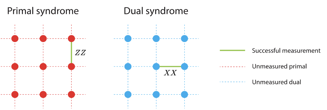
Figure 2: Examples of primal and dual syndrome graphs. The (red/blue) dashed-line represent anticipated (ZZ for primal/XX for dual) measurement outcomes from different fusion. The circular nodes denote parity checks performed on outcomes having edges adjacent to them. An edge is emphasized in black in green on each syndrome showing the ZZ and XX measurements from a single fusion operation.
Actual syndrome graphs from a fault tolerant quantum computation can be more complicated [2], but the simple examples in Figure 2 are sufficient for us to understand how a Dynamic Bias Arrangement works.
Syndrome switching
Referring to Figure 2 we see that our ability to bias a failure to occur in either the XX or ZZ measurement outcome of a fusion amounts to choosing whether the failure appears in the primal or dual syndrome graphs. We can correspondingly think of primal biased or dual biased fusions.
Figure 3 summarizes our options. Primal biasing a fusion ensures that the primal measurement outcome from a fusion is successfully measured in case of failure (at the expense of the dual) and dual biasing ensures that the dual outcome is successfully measured in case of failure . Figure 3 also includes the possibilities of complete success (which occurs 50% of the time) and a complete erasure of information due to one or more photons being lost (the primary source of noise in a photonic quantum computer), wherein both primal and dual measurement outcomes fail. It’s worth noting that loss is caused by imperfect components, rather than being a fundamental limitation of fusion’s nondeterminism.

Figure 3: Biasing fusion operations as either primal or dual, wherein we direct failures to either the primal or dual syndrome graphs. We also show the 50% chance of success (no errors) and the possibility that a photon is lost (a noise-related, rather than fundamental, error) in which case both measurement outcomes are erased.
Choosing where to fail
So how do we decide which syndrome we should bias a potential fusion failure toward? This decision rests on the fact that not all configurations of failures in a syndrome graph are equally damaging, and the impact of a new failure can depend on how previous measurement failures are clustered.
Figure 4 shows two different primal syndrome graphs with very different clusters of existing fusion primal measurement failures.

Figure 4: Examples of two damaging (left) and benign (right) combinations of fusion failures in a syndrome graph. Primal syndromes are shown, though the same distinction can be made for dual syndrome graphs. The measurement failures in the left syndrome span the grid and risk causing an uncorrectable logical error.
Though both examples in Figure 4 contain eleven failed primal measurements, the left-hand example is much more damaging. Error correction can recover from small, disconnected clusters of errors like those shown in the right-hand side of Figure 4. Far more dangerous are extended error clusters, spanning the height or width of the syndrome graph, as shown in right-hand side of the figure. These long clusters can result in logical errors that are un-correctable.
Our strategy is to use biased fusions to allocate failures in a way that avoids dangerously long connected clusters in either syndrome graph. Let’s see how this works in practise. In a real computation we perform fusions in some pre-determined order – gradually building up our syndrome graphs. This is illustrated in Figure 5, where we build out primal and dual syndromes with fusion operations from bottom to top.

Figure 5: Explicit example of choosing fusion failure bias between primal and dual syndromes to avoid the kind of damagingly large clusters of errors illustrated in Figure 4.
Recall that, when successful, each single fusion operation contributes a primal outcome (an edge in the primal syndrome graph) and a dual outcome, and in the case that the fusion fails, we can choose whether the primal or dual outcome is measured (see Figure 2). In Figure 5 we have already performed fusion operations to fill out the syndromes up until the gray line. Successfully measured edges are shown in green, and failures in black. We now come to performing a fusion with XX and ZZ measurements corresponding to the edges shown in orange. How should we bias this measurement? In other words, would we rather have a failure appear at edge A on the primary syndrome or edge B in the dual?
In this case, the decision turns out to be rather easy. The two primal graph nodes which an error at edge A would connect are already connected anyway (via the three existing failed edges shown in black). Therefore, a failed ZZ measurement at A doesn’t increase the chance we obtain a logical error in the primal syndrome. However, an error at B in the dual syndrome graph would further propagate a cluster of errors. This does increase the chance of a logical dual error. By dynamically dual biasing this fusion measurement to (so an error is more likely to occur in the primal), we therefore reduce our chance of creating an un-correctable, logical error as we continue to fill out the syndrome graphs.
Bias with exposure
It's worth noting though that not all dynamic biasing decisions are quite so easy. Consider the situation shown in Figure 6. Again we want to choose whether to primal or dual bias an upcoming fusion (so failures are directed towards edge B or edge A respectively).

Figure 6: Another example of choosing fusion bias where the optimal choose of whether to divert failure to primal or dual (at locations A or B) is not so obvious.
Looking at the previous errors (shown with black lines), either case seems to extend a cluster across the syndrome in one direction or another. In [1] we describe a heuristic called exposure, for making these tricky decisions. Exposure allows us to measure how likely it is that the introduction of a new failure into a syndrome graph will extend or join up clusters of existing failures which might cause a logical error. Exposure is inspired by the classical problem of explosive percolation [3], and assesses a candidate edge we might want to bias an error towards as follows:
For each cluster that an edge would connect to we determine its exposure by adding a 1 for every unmeasured edge adjacent to the cluster’s nodes (not including the candidate edge we are considering).
We then calculate the overall exposure of our candidate edge as the product of the exposures of clusters it would connect.
We protect edges with higher exposure (i.e. choose a primal or dual bias so that failures occur on lower exposure edges).
The idea is that by looking at the unmeasured edges surrounding it, the exposure of a cluster gives an idea of its ability to grow through future failed measurements. Then we judge a candidate edge by assessing the exposures of those clusters it’s failure would connect. For example, edges A and B in Figure 6 have exposures of 3 and 16, and so we should use a dual-biased fusion (in which failure would result in erasure in the primal graph at edge A).
With the exposure heuristic, we’re capable of making better bias decisions for any syndrome graph, even the more complex 3D graphs arising in real fault tolerant computations. In [1] we also discuss how slight modifications to our heuristic can account for other types of errors and show that the calculation and comparison of exposure heuristics is efficient and scalable.
Performance
The question of course, is just how effective is this Dynamic Bias Arrangement in helping deal with noise or imperfect physical components? Since it helps us make better decisions in dealing with error syndromes, we can hope it improves our ability to tackle noise. Though photonic components bring many sources of noise (which we have complicated error models to track), we can look at two dominant sources of noise in a photonic quantum computer:

Figure 7 shows how using dynamic bias arrangement compares to a static bias arrangement wherein we fix our choices of fusion biases from the outset (with no possibility of adapting them based on an emerging error syndrome). Our scheme is focussed on improving performance in the regime of pm and l values typical for a photonic quantum computer (the arrow labelled “Region of operation” in the figure), and also assumes one particular choice of fusion network (an architectural choice of how we layout our computation).

Figure 7: How Dynamic Bias Arrangement improves our ability to tolerate two predominate sources of noise. Shown for comparison is a static bias arrangement wherein the choice of how to bias fusion measurements is fixed. Note that this figure is also generated for a ‘boosted’ form of fusion operations – as described in 1].
The shaded regions show the maximum possible combinations of error and loss that can be tolerated with a static or dynamic bias arrangement (demarcated by the blue and orange lines respectively – which show the threshold of loss/error values, below which they can be dealt with by quantum error correction techniques). Clearly dynamic bias is more permissive – and can in fact tolerate up to 3x the loss of a comparable static bias arrangement scheme.
An actual photonic fault tolerant quantum computer will occupy some point on this plot (having particular values of pm and l). We expect our machine to operate in a regime where there is more loss and fewer errors (points lying along the black arrow in Figure 7). In this regime we come very close to attaining a 3x increase in loss tolerance. This improvement comes only from better classical decision making in the machine. The same quantum resources used for both curves shown in Figure 7.
Given the stringent hardware requirements for quantum computing, this greatly simplifies the construction of a useful device. Increased error tolerance is especially important when it comes to considering the real-world effect of errors. The well-known threshold theorem states that if errors occur below a certain threshold then fault tolerant computations can be performed. But in reality, the physical size of a machine depends drastically on just how far beyond this threshold errors can be tolerated. Thus the increased error tolerance provided by dynamical bias has a direct impact on the physical footprint and hence viability of our first useful quantum computer.
Bibliography
[1] H. Bombín, C. Dawson, N. Nickerson, M. Pant, and J. Sullivan, Increasing Error Tolerance in Quantum Computers with Dynamic Bias Arrangement, arXiv:2303.16122.
[2] S. Bartolucci et al., Fusion-Based Quantum Computation, arXiv:2101.09310.
[3] D. Achlioptas, R. M. D’Souza, and J. Spencer, Explosive Percolation in Random Networks, Science 323, 1453 (2009).